Here is the second and concluding part of the mini series on diving into the order of operations based on workout-wednesday 2022 week 15 challenge by Erica Hughes.
In Part 1 we rebuilt the solution that was in the challenge but this time our aim is to avoid using hard-encoding the maximum date or storing it in a parameter.
To recap, we want to filter a bar chart and a customer table, both displaying the top 10 products / customers in either a selected region or a selected state.
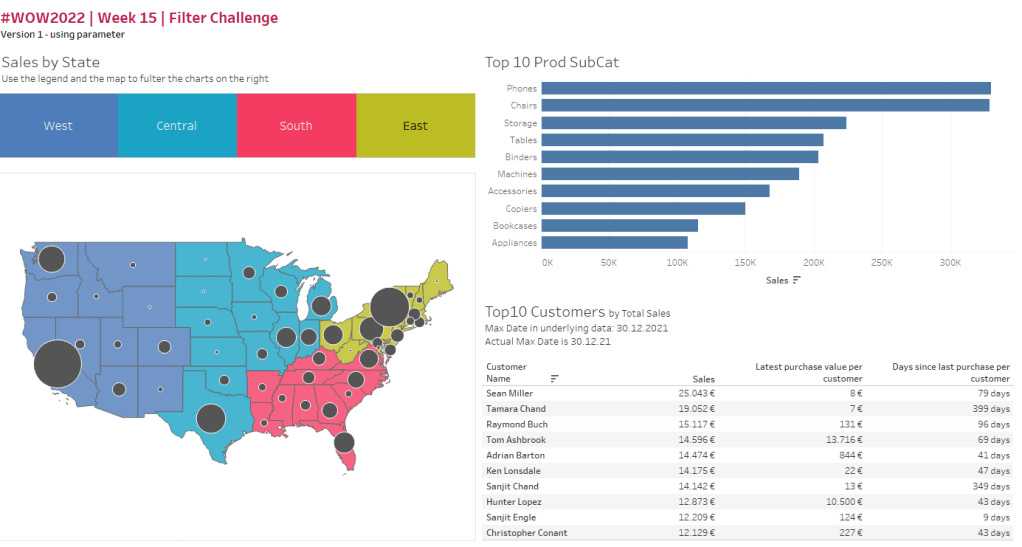
From Part 1 we know that for using meaningful top 10 filtering we need to have context filters which in turn obstructed our maximum date calculation which is why we used a parameter to store the maximum date. So, the aim must be to avoid using context filters.
Luckily, we are not all out of options. Be advised that even though the bar chart is very easy to do the table is much less so and can be more considered like a brain exercise, just playing around with the Order of Operations. I would not really advise using it as it seems to be a bit over the top.
Anyway, here we go.
Building top 10 bar chart
Again, create the bar chart but this time do not put the action filters to context, just leave them as they come (dimension filter /set level in the OoO).
Remove the top N [Sub-Category] conditional filter and replace it with either of the following two calculations
//rank
rank(sum([Sales]))
//rank
index()I will be using the first one going forward but you can use both. In case you use the latter, just make sure you order your bar chart descending.
Your sheet should look like this:
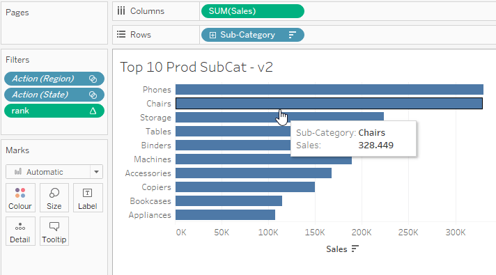
Click the rank calculation, make sure it is calculating table down (wohoo, one of the few posts on the blog w/o major changes to how a table calculation computes but.. you can also select “by sub-category”).
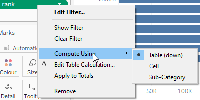
Then, click again, edit filter and filter to only show ranks 1 to 10.
And with that, we are done for this chart.
What we did is we changed our filter order. Here is an image from tableau help pages that focusses on the filters within the order of operations
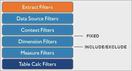
So, this time we did not move our region or state filter one step up from dimension up to context as we did in Part 1 but this time we moved our top 10 filter down the road so it now computes after the dimension filters.
So far, so good and so easy.
Now, however, on to…
The top 10 customers table
Recall that in Part 1 we had to create some calculations because for the customer table we wanted to show the days since the last purchase (max date in data set minus the date of the last purchase per customer) and the corresponding sales value of that purchase.
We used these calculations:
//Latest Purchase Date per Customer | FIXED
{FIXED [Customer Name]: max([Order Date])}
//Days since last purchase per customer
[max_date_in_dataset] - [Latest purchase Date per Customer | FIXED] //notice I have readjusted here to directly reference the LOD value instead of the parameter it feeds in Part 1 of the series. This is for explanatory purposes later on and since we want to avoid using the parameter//Latest purchase value per customer
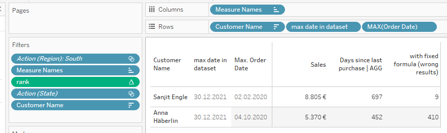
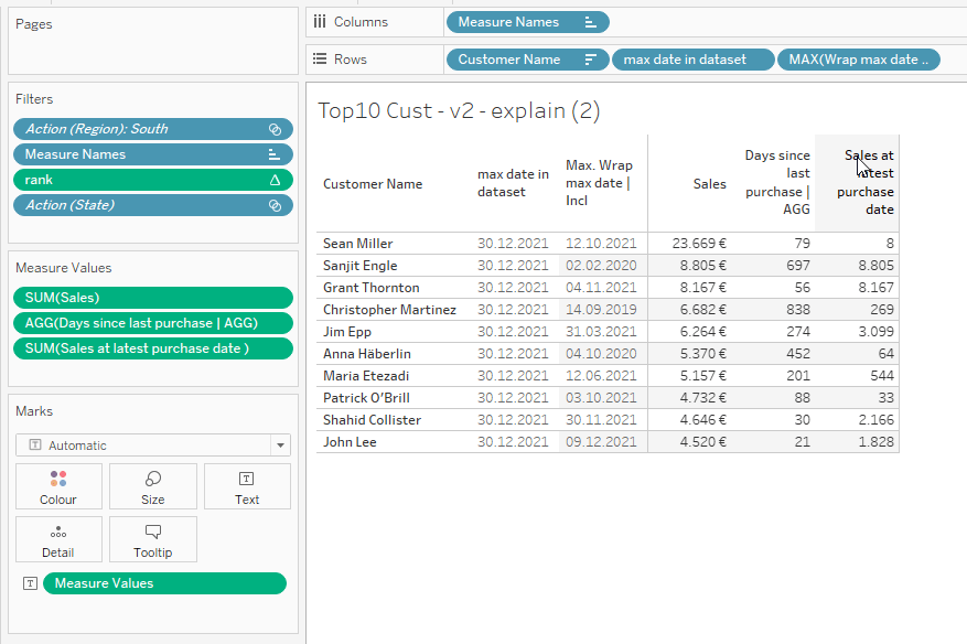
IF [Order Date] = [Latest purchase Date per Customer | FIXED] THEN [Sales] ENDOk, so let’s see what happens if we basically do the same to our table as we did to our bar chart, i.e. our filter shelf shall look like this, removing the filters from context and instead of customer top 10 filter using the rank calculation table down:
If we filter the region to South this happens
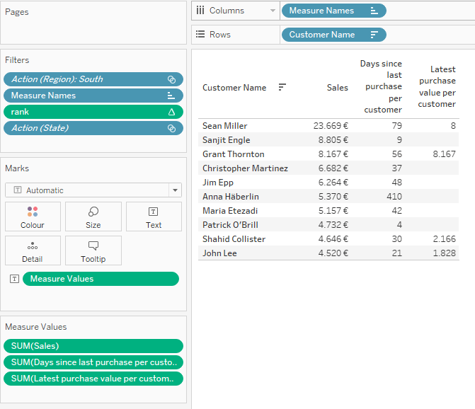
As you will notice the days are mostly false and the last purchase value per customer returns nulls for most of them. Let’s understand why.
Starting with the days since last purchase we notice that our current formula is a fixed formula which means it comes BEFORE the applied filters now that they are no longer in context. So that means we want to calculate the days since the customer made his last purchase in the South region but instead we compare it to his overall last.
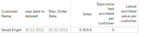
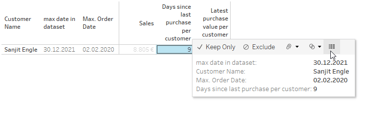
At a concrete example let us look at Sanjit Engle. His days are calculated at 9 and there is no returned value for the last sales value.
What should be returned however is 697 days and 8,805 as sales.
We can analyse his data to make sure this is correct:
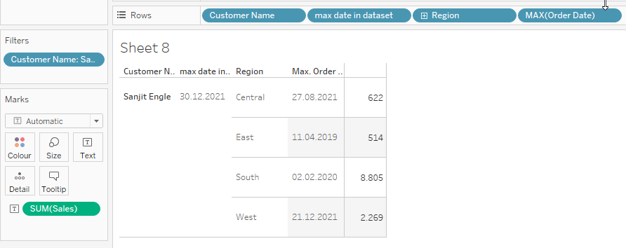
30.12.21 datediff in days to 2.2.2020, the max order date for Sanjit Engle in the South Region is 697 and the purchase value is 8,805. So this is confirmed
Going back to our table we have
Click on the 9 days (or any other measure value in the view) and click the “view data” button as shown on the next screen
On the next popup, click “orders” on the lower end
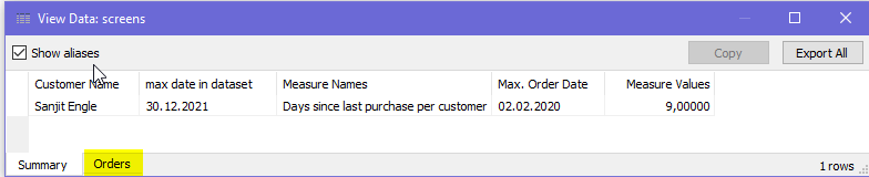
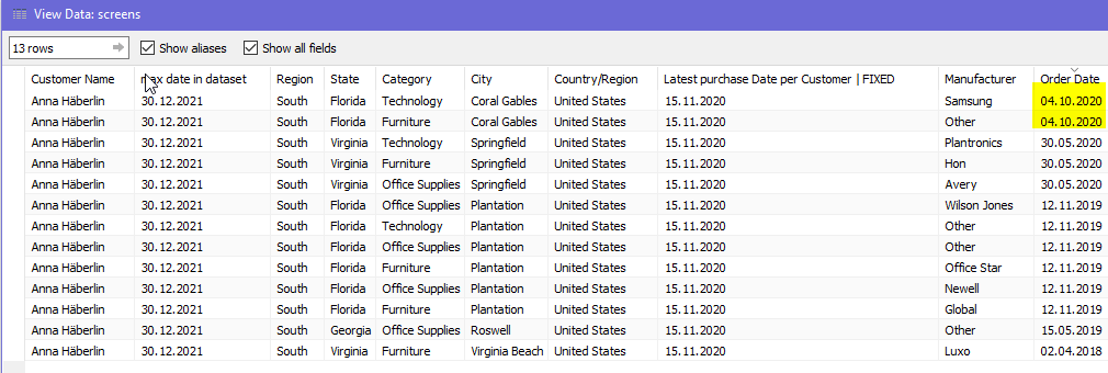
Here we get
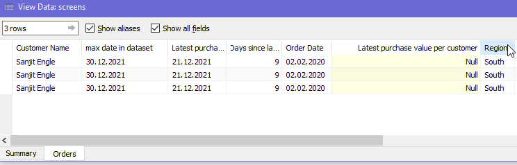
As we can see, the data that underlies our results is only three rows since it is filtered to South region. However, the latest purchase date is not from the South region but from West region (see a bit above when we had a look at Sanjit stand-alone).
The days since last purchase therefore resemble the difference of the afore two columns, which is not what we want. And the “Latest purchase value per customer” is Null because as we can see for the region the Order Date is 02.02.2020 which is not what our LOD returns so the condition of [Order Date] = [Latest purchase date] never yields true, thus we do not return any values.
Remember that in Part 1 I said LODs return like invisible columns? You will not find these in your Data Source which is clear because an LOD still depends on the circumstances (is it context filtered? Which customer are we looking at?). But you can evaluate the results of your calcs by using the “view data”. Keep this in mind, it might prove helpful.
So, what can we do?
Since we have Customers in the view (and on the view) we can simply use
//Max Date
MAX([Order Date])
to calculate the maximum date per customer since Tableau will slice this calculation along the dimension in the view, i.e. [Customer Name] in our case.
For the days since the last purchase we can do:
//Days since last purchase | AGG
max([max date in dataset]) - MAX([Order Date])
Notice that I always put the kind of calculation next to my calcs. In this case the | AGG tells me it is an aggregate calculation. We do I need to do this? Well because for every customer we want to use his max order date (after dimension filtering) , thus I need MAX([Order Date]). But my [max date in dataset] LOD returns a row level value, one fixed value. We cannot compare aggregates against rows so I simply wrap the [max date in dataset] in a max to aggregate it. Since it is one fixed value anyway, the max will return the same value. I might just as well have used min instead of max on this part.
Put this on the table and we get
697 and 452 days is correct. Looking at Anna Häberlin’s “view data” we see:
So, our formula works as intended. Great!
On to the last step
The final bit we are left with is calculating the sales on the latest purchase by customer within the respective region or state.
You might be tempted to do something like this

As you can see, that does not work because we are trying to compare on a row level. We must look through every row and check if that row’s order date is equal to our maximum order date for the customer within specified region and/or state and then return the sales.
So we somehow have to return our maximum date and make it usable on a row level. In Part 1 that is what the [Latest purchase date per customer | FIXED] calculation did.
Question is: can we rebuild that but avoid FIXED calculation because we know fixed would requires us to use context filters which led us to use the parameter which is exactly what – as a brain exercise – we try to avoid.
Let’s look at the order of operations again:
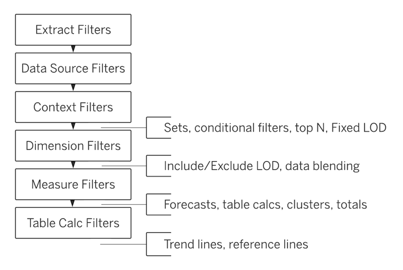
We know we are using dimension filters so we need to use something that comes after the dimension filters.
We will go and use an INCLUDE LOD and establish the calculation 1 by 1 in several steps.
We start with this
//Wrap max date
{INCLUDE : max([Order Date])}
This might look odd but all we do is to somewhat “abuse” the Include function to turn our aggregation of the max order date into something we can use on a row level, just as the fixed calculation in part 1.
We do not need to add any dimensions here because our data will already be filtered down to region or state by the action filters and the customer names are in the view already. So the max date will be calculated based on the available data after filtering for every customer.
Now we can use this in our final calculation
//Sales at latest purchase date
IF [Order Date] = [Wrap max date | Incl] THEN [Sales] END
Filtering [Region] to South gives us:
Compare this to what we did in Part 1:
Exactly the same results.
A final exercise for your understanding
As a last exercise, what would happen if we did include dimensions in our include calculation like this?
We create two calculations as before but this time we include [Region] and [State] in the include functions
//Wrap max date incl Region, State
{INCLUDE [Region], [State]: max([Order Date])}
Lets put this onto our table and aggregate once at max and once at min. Notice that I put our include w/o any dimensions as max and min and the same for the calc which includes region and state in the max and min.
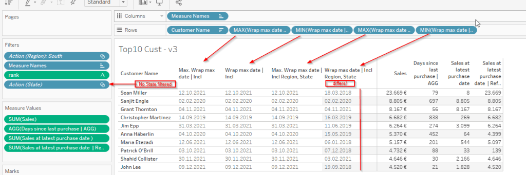
See that the min of the calculation that includes region and state differs from the max?
Why is that? And why do the other two not differ if we change the aggregation from max to min?
The reason is that in this example we have filtered the region to South but the South region still has multiple states. So the calc that includes both these dimensions will return multiple max values for every combination of region (here: South) and State (every state in the South). From this multitude of values, we then aggregate to either the max or the min by every customer which explains why we have differing values.
Our calculation that does not include [State] and [Region] returns the same values for max and min aggregation because it ignores [State] and [Region] and thus the max (inner aggregation in the formula) is applied to the entire data set that is underlying the table (i.e. filtered down to South but including all States) and then sliced by customers. Per customer, there can only be one maximum date if we do not further slice it by States or Region and therefore, the maximum of the max and the minimum of the max are the same.
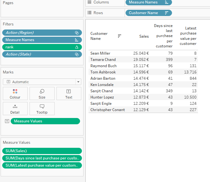
Let’s take this one step further and see what happens if we apply our “Sales at latest purchase date” calculation to the date including region and state:
//Sales at latest purchase date  | Referencing incl state, region
IF [Order Date] = [Wrap max date | Incl Region, State] THEN [Sales] END
This is a valid calculation but it returns completely different values
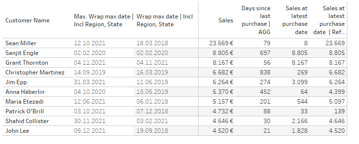
Why do we get 23,669 for Sean Miller? Again, let us make use of the “view data” feature:
Notice how Tableau offers us the Wrap max date as an independent data table and when we have a look at that we see:
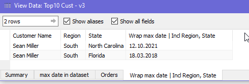
The formula returns two results; one being the maximum date for the combination of South and North Carolina and the second being the maximum date for the South and Florida for customer Sean Miller.
Now let’s look at Orders:
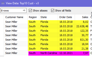
Seven orders that match South/Florida and one that matches South/North Carolina.
All these rows fulfil the condition because we are comparing the [Order Date] to 12.10.2021 in South/NC and 18.3.2018 in South/Fl, thus we get their sales values returned.
So, how would we solve this if for whatever reason we need the include to reference Region and State? Wrapping our include function into another max does not work as we would try to compare row level [Order Date] to aggregated maximum
Basically, we can use the same trick we initially utilized: wrap everything into an empty INLCUDE function
//Nested Include
{INCLUDE : max(Wrap max date incl Region, State) }
This will re-row’ify the value as only the max of the max is returned. Sticking with above, Sean Miller will return 12.10.2021 since this is the max of his max dates. And we can then use this date to check Sean Miller’s order dates vs the 12th of October 2021 and return only those sales which are 7.97 EUR / Dollars / Zloty, you name it..
IF [Order Date] = {INCLUDE : max([Wrap max date | Incl Region, State])} THEN [Sales] ENDYou might use { INCLUDE [Customer Name] } this will not change anything because we already got Customer Names in the view anyway, thus the granularity within our calculation does remains unaffected.
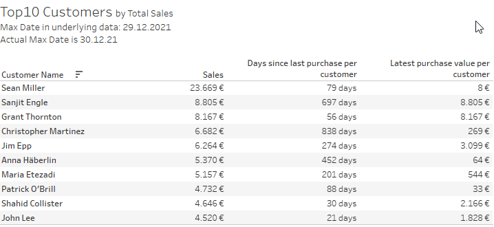
Question: Could you use EXCLUDE? Partly. If you do not add any dimensions, then yes. If you go for {EXCLUDE [Customer Namer] } then you will get completely different results.
For the South region, your Latest purchase date will return 29th of December 2021 even though none of your top 10 South region customers has this date as his maximum order date.
Reason: we exclude the Customers from our calculation and are still filtered to the South region. So a calculation like this
//Excluding Customer Names
{EXCLUDE [Customer Name]: max(Wrap max date incl Region, State) }
will return the maximum date for all customers of the South region. Since our rank calculation that we use comes after the EXCLUDE calculation in the order of operations, we just do not see the customer that “provides” the 29th of Dec 2021 as the max date for South region. Tip: the date stems from customer “Katherine Hughes” who ranks 54th in the South region.
Question: could we use FIXED? Haha just kidding, not going to reiterate that. Just re-read from the top if this has remained unclear.
And that is it, now you hopefully have gained a bit more insight into the order of operations and a bit into Level of Detail calculations.
If you want to follow along find the accompanying workbook on my Tableau Public.
As always I hope you found that useful and I appreciate your feedback.
Kind regards
Steffen

Leave a comment