The challenge
Just as I had finished my blog on how to transfer results of a table calculation from one sheet to another, a new but related question popped up on the forums.
This time, the user wanted to compare two independent rankings. I.e. he did not want to compare on a product level but instead he wanted to compare Rank#1 from Ranking A to Rank#1 from Ranking B etc where both rankings could be based on completely independent filters.
So contrasting the previous blog, this time we do not transfer dimension results but rather the actual measures that are derived in Ranking A to Ranking B.
Sounds tricky? It was.
Be advised we will be using table calculations a lot and in order to derive the result always make sure you have set the calculation correctly (it is not difficult but just make sure all is in order).
Let’s get started
As per usual, data set to be used is Sample – Superstore.
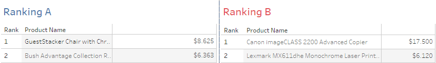
Start with creating the two rankings. Ranking A and Ranking B. On both we use Region and Segment as filters. Put both of them into context. Do not sync the filters between the sheets, they must be independent since we want to have independent rankings.
Next, put product names on the filter and filter by Top N by Sum([Sales]). The Top N can be fixed or be set via a parameter, up to you. Sum of Sales goes on Text marks and Product Names on the rows shelf. Finally, feel free to add a rank before the Product Names by either creating a rank calculation or simply using an index() calculation, put it to discrete. Done.
Important: do not use rank filtering by a rank or index calculation as these only hide anything that does not match but data will still be in the view, though not on the view. Also, make sure you order by Product Name based on sum of sales descending.
This is what it should look like

The transferring sheet
Preparation
Now what we need to do is create a sheet that will enable us to transfer all results from Ranking A to a Deviation Sheet.
In order to do so, what we need is (note I have split some fields to make it more understandable):
- A string parameter, name it p.StoreValues
- An integer parameter which we name p.Store Max Length
- a total of five calculated fields as per following
//align string length
/* --> this calculation will transform the calculated value per product from Table A into a string of equal length by adding spaces to fill the difference in length per string compared to the longest string */

IF LEN(STR(ROUND(SUM([Sales]),0))) < WINDOW_MAX(LEN(STR(ROUND(SUM([Sales]),0))))
THEN
    STR(ROUND(SUM([Sales]),0))
    + SPACE(WINDOW_MAX(len(str(round(sum([Sales]),0)))) - LEN(str(round(sum([Sales]),0))))
ELSE
    STR(ROUND(SUM([Sales]),0))
END
Note that I remove decimals as this would overcomplicate things. So, if you are comparing sports’ results that differ by the milliseconds, maybe this approach is not for you (or needs adaption).
//delimit aligned strings
/* --> this calculation replaces the spaces we inserted above with a hash and adds a final hash, thus delimiting our measure values */

REPLACE([align string length],' ',"#")+"#"
Next, the formula you might recall from the previous blog post
//total_string_to_parameter
PREVIOUS_VALUE(([delimit aligned strings]))
+
IF CONTAINS(PREVIOUS_VALUE(([delimit aligned strings])), ([delimit aligned strings]))
THEN ""
ELSE ([delimit aligned strings]) END
Finally, let us get the max value of the total string that we want to pass to the parameter
//transfer long string
window_max([total_string_to_parameter])
With this out of the way, we need one more calculation
//Max string length
WINDOW_MAX(LEN(STR(ROUND(SUM([Sales]),0))))
Wait, didn’t we use this formula above already, why not reference this one? Honestly, I wanted to but Tableau threw one of the famous “k t” errros. No idea why, didn’t bother. Maybe it is working fine on your end, give it a try.
A general note: You might be wondering at some places why this seems to be done so complicated and not using regex_replace() or findnth() formula. Reason is: all these formulas that indeed would simplify life do not work with table calculations. Will explain later on in more detail.
Moving to the actual sheet creation
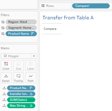
Now with everything being prepared, create the sheet “Transfer from Table A”. Set filters from your Ranking A sheet to be applicable also to the Transfer from Table A sheet.
On the details, put
a) Product Name (sort descending by sum of sales!, this is very important),
b) transfer long string, set to compute using Product Name
c) Sum of Sales
d) Max String Length, compute using Product Name
On rows, put an ad-hoc calc named “Compare”; set marks to polygon.
Create the Delta Sheet
Preparation
Now, we need to prepare our delta sheet, so create a new sheet, name it Deltas, Table B as Base.
Create three calculations:
//index -1
index()-1
//Delta
[return values from table a] - SUM([Sales])//return values from table a
FLOAT(
LEFT(
MID([p.StoreValues],[index -1] * [p.Store Max length]+index(), [p.Store Max length]+1),
FIND( MID([p.StoreValues],[index -1] * [p.Store Max length]+index(), [p.Store Max length]+1), "#",1)-1
)
)I guess the last one needs some explanation. What happens is we want to extract the string that actually forms the number from our parameter and we want to do that row by row (i.e. in row one we want to extract the first value, in row 2 the second and so on). This part
MID([p.StoreValues],[index -1] * [p.Store Max length]+index(), [p.Store Max length]+1)does that. We extract from p.StoreValues with starting reference being our row number less one times the length per string plus the row number and we take the next lenght +1 chars.
Example. Imagine our parameter has only two values stored (Top 2 selected) and the values are 17000#5600##
The p.Store Max Length parameter would bear the value of 5 (which is the max length of the values prior to delimiting it). Now, we are in row 1, i.e. index is 1. The formula would evaluate to
MID([17000#5600##],0 * 5 + 1, 5 +1)So, take from the total string, starting at 1 the next 6 characters. So we would get 17000#
For the second row we would get
MID([17000#5600##],1 * 5 + 2, 5 +1)This translates into “take from the total string, starting at 7 the next 6 characters. resulting in 5600##
You now also understand why we can’t use findnth or something because in order to define “which nth” we need to pass the row number. Which is the index(), which is a table calculation which does not work with findnth(). So, there we have the reason.
Obviously, we do not want the ## in our results since we need numbers to compare. That is we wrap this into a left() calculation. The first part of the left calculation is the above which returns what we just analysed. The second part defines how many characters we want to extract
//second part of the LEFT() formula, after the comma
FIND( MID([p.StoreValues],[index -1] * [p.Store Max length]+index(), [p.Store Max length]+1), "#",1)-1
Here, we find the position of the first delimiter, i.e. the #, but obviously we cannot always go from start/the entire string which is why we repeat the MID formula that will give us the string that we analyse. The substring that we search is “#” and the starting reference is 1. When we find that position, we substract one.
So in the example of our second row, the first part resolves in 5600##. From there, we start from the first character and find the first # at position 5. From this 5 we subtract 1 and get 4. So now we have
LEFT(5600##, 4)which yields 5600.
Since this is still a string, we wrap everything into a float and voila, there we go. We have successfully extracted per row our values from the parameter and can now do the Delta calculation.
Create the sheet
With all the preparation out of the way, create the sheet. This time, make sure that the filters are coming from your Ranking B sheet (since Ranking B is our base).
Put Delta on Text marks, Product Names go on rows. Make sure to sort Product Names by sum of sales descending! Compute Delta table down.
Since your parameter is still blank, you will not see much. So lets move to the dashboard and put everything together.
Create the dashboard
Put Ranking A and Ranking B into a horizontal container next to each other. Put Delta sheet next to Ranking B; align everything.
Put the filters for Ranking A and Ranking B on the sheet.
Finally, put “Transfer from Table A” sheet on the dashboard. Hide title. You should be left only with the “Compare” Button.
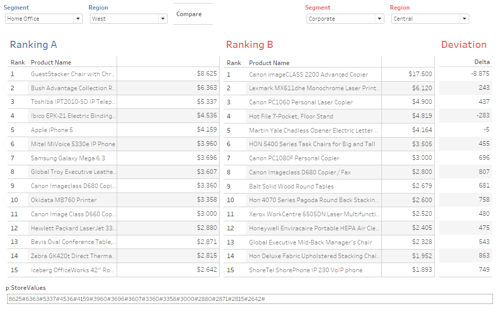
For testing purposes, feel free to show the p.StoreValues parameter (its not needed on the DB but might help to visualize).
Create two parameter actions:

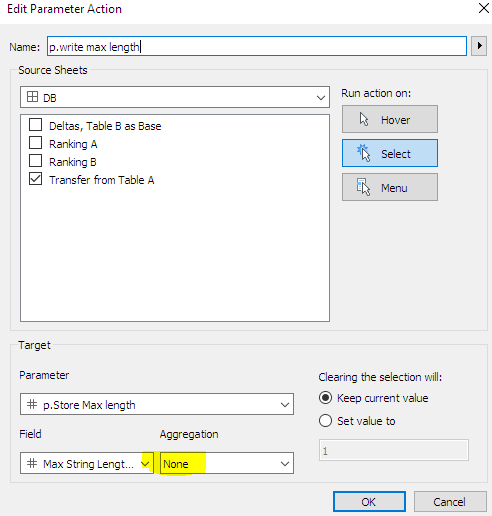
Here are two screens of the final result. Parameter included for clarification only.
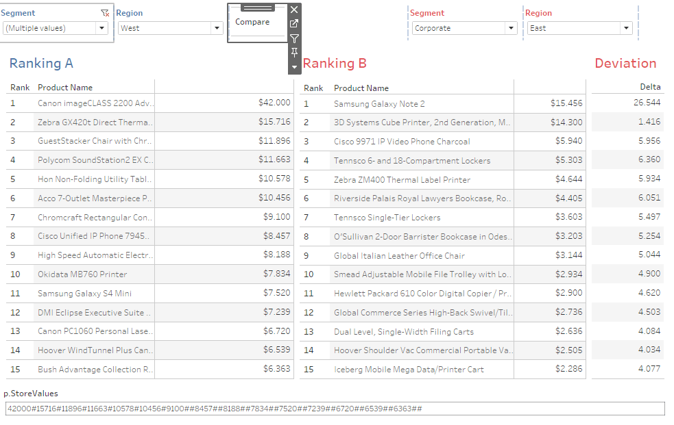
Caveats
This solution requires the user to press the “compare” button after he has set his filters for both sheets so make sure to guide him accordingly.
The Top N should be set to be the same for both rankings. If Rank A only has 10 results but B has 13, this will get you in trouble. (as a quick idea, create a parameter that takes the Top N count from A and compare that to Ranking B index(). IF Index() exceeds the parameter, show null. Didn’t test so far).
And that’s it.
As always, if you’d like to follow along feel free to download the file from my Tableau Public profile here https://public.tableau.com/app/profile/steffen2460/viz/comparingtablecalcsfromtwodifferentsheets/DB#1
Thanks for reading and I appreciate your feedback.
Until next time
Steffen

Leave a comment