Mastering Table Calculations Pt. 1: From Basics to Advanced Settings

In one of the recent episodes of Workout Wednesday – Week 15 2024 – Tableau Visionary Hall of Famer Andy Kriebel posted the challenge to create a quite dynamic Trellis chart.

As there were some details to be considered this made me think of creating a mini series on the topic of table calculations which concludes with a practical application, based on the WOW challenge.

In this Part 1 we will go deep into table calculations, followed by an excursus on data densification in Part 2 and finalised in Part 3 by applying our learnings to WOW2024-Week 15.

This series will hopefully equip you with a better understanding of the intricacies of table calculations, especially their advanced settings that are rarely used and enable you to understand two possible options to overcome one of the problems within the challenge posted by Andy Kriebel..

Since this first part is rather long see below a table of contents so you can jump right where you feel like you may find the info you are looking for.

Let’s get right into it.

Table calculations – what are they? And where do we find them?

Table calculations form their own layer of calculations within Tableau. They are based off of aggregated results from a earlier stages within the order of operations. As an example, let’s say you want to compute running total of your sales, then the calculation will look like this:

To derive such a calculation. you drag your date field to columns and the sales measure field to text.

Tableau will automatically aggregate the sales as sum[sales]) .

Now you can turn this into a table calculation by either clicking the small triangle on the right of the sum([sales]) field or right click it and click “add table calculation” or below that the “quick table calculation” where you will find several pre-defined calculations.

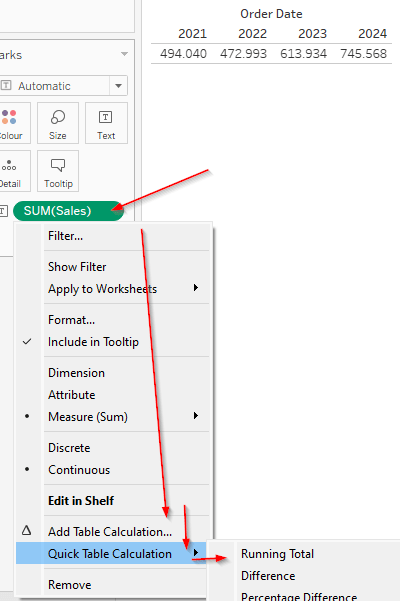
Tableau will then first send the query to the database for the sum of sales. Something like

SELECT 
  extract(year from order date) as year,
  sum(sales) as sales
FROM source
group by 1

Thereafter, the Table Calculations will be performed within Tableau. You will not find any query being sent.

Tip: When you double click the created table calculation, you can coyp and paste the formula or, even better, simply drag it onto the data pane whilst keeping ctrl pressed. This will give you a new field that you can have a look at to understand how Tableau creates the predefined calculations so that you can adjust them if needed.

Table calculations can be identified by a small triangle on their right end of the pill. However, personally I would recommend to always name your fields clearly to state that they are table calculations. Something like [Running Sum of Sales | TC].

The below gif summarizes the discussed basics on how to create a table calculation.

Table calculation basics

Compute using

Tableau offers a multitude of options how you setup your calculations to work and you can also set them independently if you nest them.

We can use one of the predefined options or go into edit table calculations where we are greeted with yet another round of possible layers.

I will not go deep into the above options in detail as they are pretty straight forward but here are some general comments.

The red part, i.e. everyting, is what forms the table. The green highlight shows what is considered a pane. If you select “down” for either table or pane, the calculation will run within the table or the pane by each column. If you select across, it will run across the entire row, again either for the table or the pane. Down and across or vice versa then combines these two basically creating an either Z-shaped or an inverted N-Shaped approach to calculating.

What you should remember here is that:

Options are computed based on what you (visually) got as a table on your screen, based on columns and rows. I.e. your layout in Tableau defines the table along which your table calculation is computed.
Lookup(sum([sales]),-1) will give you the result of the preceeding cell where preceeding is dependent on how you set your calculation to run (across implying your preceeding cell will be the one to the left and down implying your preceeding cell will be the one above your current cell).
This also means that the necessary partitions are automatically created by Tableau by position where position means the position within your (visual) table.
Any options below “cell” on the compute using screenshot above are based on the dimensions you have ON the view (not necessarily IN the view. I.e. it will also offer dimensions from the color or detail shelf and even the pages shelf. Not only those that are on rows and columns).
Selecting one of these options will set the selected dimension as the addressing dimension whilst all others will be used to form the partitions.

Addressing and partitioning

Addressing means the direction in which the calculation moves and therefore the order is relevant. Addressing fields can be identified by a tickmark when going into “edit table calculations”. Order of addressing fields defines the order how they are considered within the calculation, usually referred to as going top-down (though I personally like to think about it bottom up as you will see soon).
Partition in turn define sub-tables within which the calculations are performed. They therefore also define the boundaries for the calculations and restart the calculation once the end of such a sub-table has been met. Partitioning fields are defined by being unchecked and the order does not matter.
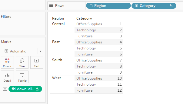
- Example: a calculation that has Region and Category as the partitioning fields and Ship Mode as adressing will calculate (lets put this in words) “for every combination of Region and Category (North – Furniture would be a sub table just as Central – Technology) calculate my [index…] along Ship Mode.”
- This also explains why the order does not matter as Central – Technology comprises the same data as Technology – Central.

Example for partitioning by category and region addressing ship mode.

For another practical example of partitioning you can refer to this blog post I wrote in 2021 which also shows the sub-tables created by partitioning.

Digging into the rabbit hole

Edit table calculation

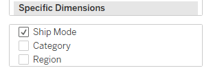
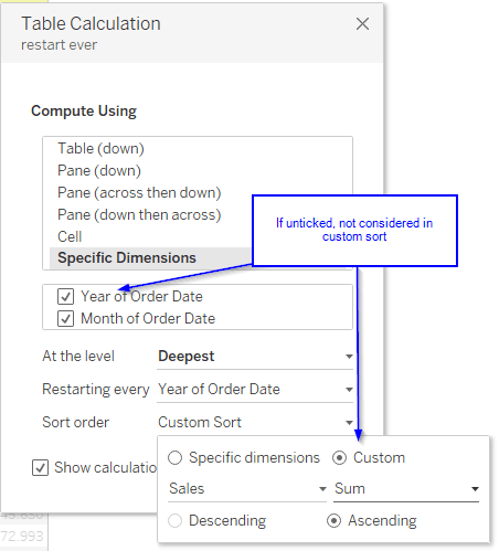
If we go into this segment, this is where the magic happens. The new option we get is “specific dimensions” and if we select that, we get to choose our own partitions and addressing.

Notice how – on selection of one of the other options – Tableau will also show the partitions and addressing fields by (un-)ticking them correspondingly.

In this part, we are now free to break away from the visual outline of our table and create partitions that are based on value instead of position. This is useful for example whenever your requirements are to calculate something that is not within the realm of the predifined options.

Here is an example:

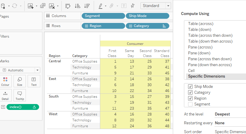
Have a look at the following example. The indexing (running numbers from 1 to 48) seem to be very strangely positioned.

That is because I have selected the Segment to be the partition and addressing going from Ship Mode to Category to Region.

We take the first Region, Central and the first Category, Office Supplies and the first Ship Mode, First Class, and index this at 1. Then, On to the second Region, sticking with first Category and first Ship Mode, assign 2 and so on.

After we have done same with the last Region, we are back to first Region but 2nd Category , first Ship Mode. And so on it goes.

For me I therefore like to think about the way it is calculated not top down for the addressing but rather bottom up. You will find “top down” though quite often when addressing is described.

On the next screen, the index is shown using “table down” from the quick selection whilst the calculation named “edit tc” (which is also just a renamed index) is also going table down but I have swapped the addressing fields so that they no longer correspond to the layout of the table, i.e. “edit tc” field is going from Category to Region instead of following the layout which is going from Region to Category:

Further, be advised that once you have setup your table calculation using specific dimensions, adding dimensions to your view will result in Tableau considering them as part of the partitioning!

Understanding the effects of partioning and addressing order

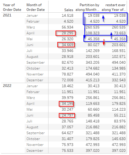
Let us have a closer look at that. In the next screen, I am using two index() calculations but set them differently. Both are partioned by the year and both use the same addressing fields but in a changed order.

The first index goes from the Instagram handle to Month whilst the second one does it the oppositve way, meaning I have placed the Instagram handle ABOVE the month in our “edit table calculation” setting.

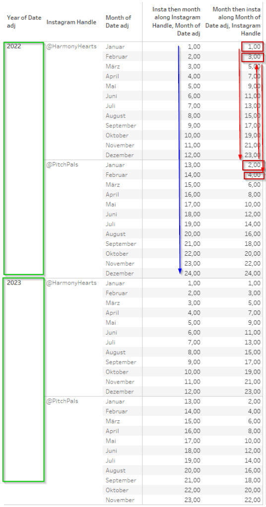
The first thing we notice is that both calculations basically “reset” at the year 2023. That is because our partitioning is set on the year, so each year creates its own sub-table with the data in it based on which the other calculations are being done.

The blue arrow shows how the index increases by +1 when going from Instagram handel to month. Since Instagram handle is placed above month in the addressing, we first go into the first option of the instagram handle and then compound by every month therein, then transition to the next handle and keep (this is important, we are not resetting!) incrementing again for every month.

For the red boxes, we can see that it works differently here. Since month is our higher-up addressing field, we first go into the first month, here January and then increment this based on the two instagram handles we have. Only once we are done with this, we now to back to the next month, February, where we continue to increment again for both instagram handles and so on and so forth.

At the level

At the level is only available when you have at least two addressing fields selected.

In this case, it will offer you the two options plus the default “deepest” selection.

Keep in mind that “deepest” is nothing else than the bottom-most option of the selected addressing fields. I.e. in the above screenshot, it does not matter if I select “deepest” or “Region” as the Region IS the deepest. There will be no change to your results.

At the level basically allows you to re-introduce a “by position” layer even when using specific dimensions. It creates another partition by position.

Partition by position explained

Indeed, the “by position” in this regard can be quite confusing. Didnt we just say that “edit table calculation – specific dimension” is meant to break with the visual outline (and therefore position) of our table?

I hope the following example clarifies.

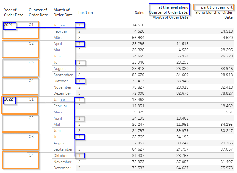
On the left you will see monthly sales and a lookup of the previous value via lookup(sum(sales),-1) which is set to be “at the level” of the quarter. Also, we partition the table by the year.

The right hand table then shows you the table that is basically being constructed underneath when using at the level at the quarter.

It highlights how tableau groups the rows based on their positions (aha!) when calculating at the level. Let’s dive into it:

Every row within a quarter has a position as I outline. The lookup() calculation that is applied is set to look up the previous value one row above. On the left, it looks a bit strange because the first few rows are empty for our lookup. But notice that Q2, April, looks up the value of Q1, January at 14,518 USD..

(1) Now this may seem odd on the outside as we only wanted to look up the value one row above lookup(sum(sales),-1) . which should imply that we look up March (“März”), shouldn’t it?

(2) However, notice that the POSITION of April AT THE LEVEL of the quarter is 1 and so is January for Q1. If we now transform our table to be ordered by the position, then we see that January, April, July and October all are at position 1.

Therefore, WITHIN our Position 1, one row above from April is January.

(3) Look also closely on the right again and you will notice that the calculation resets on Position 2 after Position 1 is done. This can be recognized by the fact that February has no value because there is no preceeding row.

The fact that the calculation resets every position and also that we can visually observe that the calculations are performed WITHIN each position, this underlines that indeed the positions form a partition!

The difference between “at the level” by position partitions and by value partitions

Ok so we have established that at the level creates another partition by position but would that not mean that I can do the same just by unticking whatever I need as my partition? I.e. does “at the level” mean the same as just unticking a box?

Well.. not exactly. Let’s have a look.

The orange highlighted bits are the standard “specific dimension” settings for partitioning using the year and the quarter. Any calculation is done within those partitions.

Remember, partitioning by the year and then setting “at the level” to Quarter does NOT create a partition based on the quarter. It rather creates a partition based on the position of the relevant row calculated at the level that we defined, here the Quarter.

If we were to add the days to the view, then we STILL would be computing based on the positions within the quarters but now the months and days would define the relevant position within the quarter (Important: on the following screen, the position is not entirely correct and is only in there for easier reference).

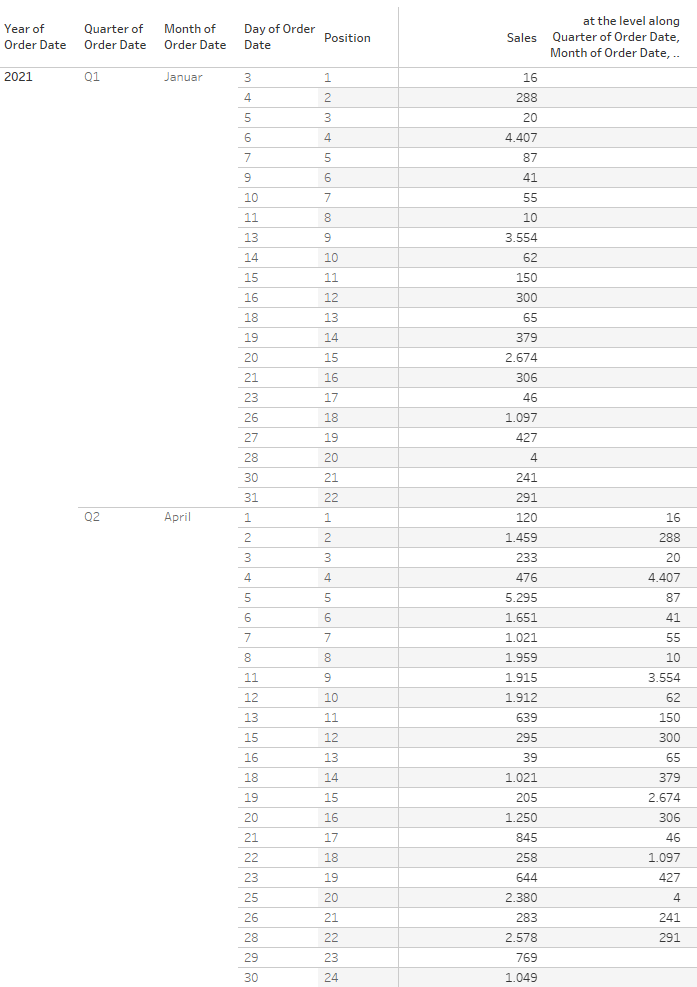
Take note how the last two rows in April have no values because there is no position 23 or 24 in January.

Further, it is very important to keep in mind that position clearly does not mean “same value”. In April, Position 1 is also April 1st. However, the January value we compare it to is not January 1st but January 3rd which is the first position since there is no data for Jan 1st and 2nd.

Understanding positions

Above, we had dealt with quarters where it is somewhat intuitive that the preceeding quarter of Q2 is Q1 and we then compare the first months within each against each other.

However, there can be cases that are less intuitive and as was stated before, my position calc in the previous screen was not entirely correct.

On the following screen, we are again using “Category” as our at the level.

Things are looking quite ok from the outset but have a closer look.

Corporate in Technology shows the values from corporate in Office Supplies but since there are less rows in Technology – Corporate than in Office Supplies – Corporate, we are missing the last value (and our values are assigned to different types of ship mode which is ok given how we calculate but please consider this when using at the level! you deal with positions here, not dimension values).

Now one might conclude that Home Office then should go on and simply take the last, missing value from Corporate but it doesn’t. It starts anew and takes the first value from Home Office.

This tells us that the positions are not calculated table down within the addressing fields that follow the at the level field (i.e. we cannot position office supplies at 1 to 12 and Technology at 1 to 11) but it is rather a mixture where every part gets their position.

What I mean by that is that Segment gets a position and Ship Mode gets one. So instead of 1 to 4 for Office Supplies/Consumer/Ship Mode we would rather get 1-1, 1-2, 1-3, 1-4 and the same for Technology/Consumer/Ship Mode.

For the Corporate bits we would then get 2-1,2-2, 2-3, 2-4 on Office Supplies but only 2-1, 2-2 and 2-3 on Technology.

Finally, for home office we get the 3-1, 3-2, 3-3 and 3-4 for Home Office as well as Technology and thus the lookup works again.

This is what it would look like in a table:

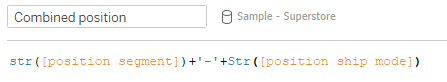
If you want to create this position in your own calculations what you will need is one index claculation per addressing field that is coming AFTER your at the level field. For each of these, partition on all other dimensions EXCEPT for the one you are at. So for Segment, I partition on Region, Category and Ship Mode and use Segment as the only addressing field.

For ship mode the same, just swapping ship mode and segment.

Then, combine these fields like this:

Increments “At the level”

Let’s have a further look at how index increments work at the level.

Here, I am using two indexes once again, one just going table down which means every dimension is selected as the addressing field. On the second column, I am doing exactly the same but am setting the Category as my “at the level”. Notice the difference:

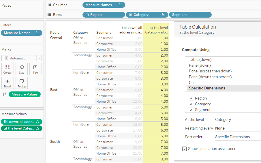
Whilst the table down just increments +1 for every row all the way down, the “at the level” calculation does not do so. It basically ignores anything that is below the selected “at the level” option. Thus, in this example “Segment” is being ignored whilst incrementing.

Contrasting, Region which is above Category is contributing to our incrementing (otherwise East – Office Supplies should show 1 instead of 4).

You get the same results for the index as if the Segment field would not exist in the table at all. See here, same results index-wise but with fewer rows as we miss the Segment. This behaviour persists regardless of the number of addressing fields that are positioned after the “at the level” field.

This behaviour is apparently quite different to what we saw when having a look at our lookup calculation. However, it holds for size(), first(), last() and the index() functions.

Restarting every

Restarting every… is an option that allows us to set yet another break within our calculations. It has quite some similarties with just setting the partitions as those also stipulate the boundaries our our sub-tables and therefore restart the calculations on every new combination of your partitioning dimension members.

Contrasting to this standard approach. restart every allows you to keep a dimension as part of the addressing as well as partition by it.

What’s the use case?

This suppossedly will come in handy whenever you are in need of specific sorting. An example would be the following:

Imagine we have only two dimensions in our view and for whatever reason we want to show a running sum that accumulates not across the standard order of the dimension members but from smallest to largest, but breaking/restarting (i.e. partition) on the year.

The problem we face is that when partitioning by unticking, that dimension is no longer considered in a custom sort.

The next screen illustrates the problem.

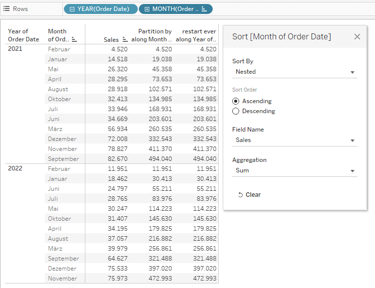
The middle column shows the unticked partition by option whereas the right hand column shows the effects when using the restart every option and both using a custom sort on sum of sales ascending.

The partition by column goes from February to January to May and then to June whereas the restart every column goes from Febuary to January to May to April.

The reason is that on the first column the year is not available for the sorting, thus the months are sorted by their OVERALL value and here, adding April value for 2021 + 2022 is 62,491 whereas June is 59,467.

Since we partition by year, the summed values are still only those of the year 2021 or 2022 respectively but not jointly.

Therefore, within the partition logic sorted by custom sum of sales, June comes prior to April because we do not consider the year. If we consider the year, then in 2021 April value clearly is less then June value and therefore, April is added in our running sum prior to June.

Personally, I find such a case super edgy and I have yet to come across a usecase, especially when considering that I could achieve the same results by simply changing the sort on my months in above example by right clicking, selecting nested and in my table calculation keep the sort on “specific dimension”.

Yes, this would change around my months (notice that the months are now ordered by their individual sales within the month ascending) but does that not automatically give more insights and make it much easier to read? I think so.

Anyway, let’s move on to our final bit for today.

Nesting table calculations

We will finish this posting with a short look into nesting table calculations.

A nested table calculation is a table calculation that comprises another table calculation.

It is important to note though that this does not mean a calculation where we write everything at once like

// not really nested
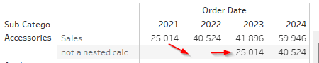
lookup( lookup(sum([sales]),-1) ,-1)

This calculation will rather stack than nest. As the next screen shows we can see that the lookup stacks: the 25k are shifted by 1 column and then another one since we lookup the lookup

In contrast, a nested calculation is build by creating one calculated field and then the next one where we reference the first calculation within the second.

Sticking with the previous example we can do:

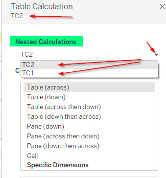
// TC1
lookup(sum([sales]),-1)

//TC2
lookup([TC1],-1)

We can then drag TC2 and are now able to set two different ways of computing, if we want to.

This way, we can lookup diagonal if we like by setting TC1 to go across and TC2 to go down for example. This gives us a diagonal lookup.

And with that, we are done for today.

Quite a lot to take in. Give yourself a round of applause if you made it here.

Some words of Acknowledgement

I would like to acknowledge some true “Giants of Table Calculations” that have done work on this as far back as 2012! Long before I had even heard of Tableau, let alone Table Calculations.

So, thanks to Jonathan Drummey and Joe Mako.

Please if you haven’t done so check out Jonathan’s blog on drawingwithnumbers.artisart.org

In Part 2 we will be doing a quick excursus on domain padding and domain completion which will be helpful in understanding the options we will discuss in the final Part 3 of this series.

And that’s it for today. I hope you found that useful.

As always appreciate your feedback.

Until next time.

Steffen