Mimicing Excels sumif / Vlookup without data manipulation

Update 23 November:

As some have noticed, would it not be easier to just do a

window_sum(sum[hour_hours]))

and compute that by

Answer is: yes. The original question was phrased differently with the user asking to also deduct several values which, in retrospect was not what he wanted. All he wanted was to just sum the hours for every office_id which we do with the above by partitioning on hour_office_id and addressing office_id which translates to

for every hour_office_id by office_id give me the sum of hours

Original posting:

A recurring question on the Forums is when users ask how they can mimic the excel vlookup or a derivative formula to that effect such as a sumproduct or a sumif.

Usually, this means duplicating the data source or in some cases using LODs but for today I want to show how we can – at least in some cases – achieve the desired outcomes without self-joining your data by just using the all time favorites (and so often completely overlooked) table calculations (I really should rename this blog to tableau table calculations).

The question

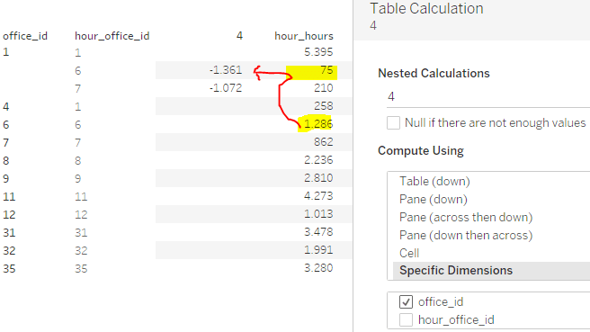
So, here is the request that was asked: In column 1 of the data the user has office ids and in column 2 there are the ids of offices in which working hours were actually booked. The measure in question then represents the booked hours.

The user wanted to know how he could sum all hours per office id (column 1) which means including values from other office ids where the “booked office id” is the same as the office id in question but also, removing the office hours that did not belong there. See below screenshot to clarify (also, keep this layout in mind when later on discussing the table calculation settings):

So office_id 1 should have 5,395 + 258 – 75 – 210 = 5,368 hors. Office_id 4 would be zero / removed and so on.

Now this may seem easy on the outset but remember, Tableau isn’t Excel. It is not a cell based tool but operates over a (set) of data. We are dealing with row based data here which means at the above example that we have rows where office_id =1 and hour_office_id is 1 r 6 or 7.

But how do we tell the row in which our office_id 4 reside that we need it’s value to be attributed to office_id 1? How to aggregate row values that (seemingly) have no connection because the connecting values reside in different columns?

In Excel, this is easy. Copy column 1, remove duplicates, create a sumproduct or even easier a sumif that sums all hours when the column 2 equals the jde-duplicated column 1 and that’s it.

But across data bases, this is less easy.

Getting there in six steps

To achieve what we want we will create five calculations (that boil down to one, it is just needed for being able to set all the compute directions) and one filter.

First, we calculate a simple rank

//1. Rank
RANK_DENSE(min([hour_office_id]), 'asc')

Next, we get the first nest calculation by computing the window_min of our rank calculation.

//2. Window Min Rank
window_min([1. Rank])

Though it is not needed, it is always advisable to put these fields onto your table and set the compute directions immediately. This way, you can make sure everything works as expected and when putting the final calc in play, you know how to set each nested calculation’s partitioning and addressing.

//3. Window Sum
if [2. Window Min Rank] = [1. Rank] THEN window_sum(sum([hour_hours])) END

Calculation 4 is basically the inverse of calculation 3, i.e. we subtract those hours that should not be booked within the respective office id (notice I put the minus up front, just in case you overlooked that and wondered where it is)

//4. Negative Window Sum
- if [2. Window Min Rank] <> [1. Rank] THEN window_sum(sum([hour_hours])) END

Calculation 5 then bringts everything together:

//5. Result
window_sum([3. Window Sum]) + IFNULL(window_sum([4. Negative Window Sum]),0)

Notice that the final calculation, by including calculations 3 and 4, also includes calculations 1 and 2, so we need to make sure to set all partitions and addressing correctly.

Setting the calculations rights

Calculation 1, Rank, can just be left to compute table down. Note how this will result in the rank be computed by office_id and by hour_office_id:

Calculation 2, Window Min Rank, is set to partition on office_id and address hour_office_id:

This results in:

For calculation 3, window sum, we invert the above, i.e. we partition on hour_office_id and address the office_id which results in:

Notice here the highlighted parts how Tableau puts together the hour_office_ids because we partition on this field.

For calculation 4, the negative window sum, (i.e. those parts that we need to subtract) one might be tempted to think that this should be exactly the same as for calculation 3 but it isn’t! Why is that?

Let’s have a look at what happens when we set it up just as formula 3:

we can see that Tableau (correctly) partitions on the hour_office_id and applies the window sum on that (negatively that is). But this way, we get the effect that Tableau subtracts the entire value which is not what we want, we only want to subtract those values, where office_id is not equal to hour_office_id.

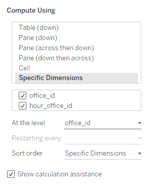
Luckily, Tableau offers another partitioning option by selecting “at the level”. So let us keep both fields, office_id and hour_office_id in the addressing and then partition via “at the level” on office_id. Also: It is super important that you pay attention to the order of office_id and hour_office

Wait, why would I first NOT partition on office_id (or hour_office_id) and then again partition on this field?

For this we need to understand that anything that is not “specific dimensions” we partition by position (i.e. the way our viz is structured / how the pills are positioned).

When we use specific dimensions, we can basically break the connection between visual layout and the way we compute. Using “at the level” then re-enables the partitioning based on position.

In our case, we have office_id and hour_office_in in our scope as the addressing fields, i.e. the calculation is done by office_id and by hour_office_id.

When we now set “at the level” to office_id, we “break”, i.e. restart the calculation at the office_id level. Note that the order is very important as stated before, i.e. we need the calculation to move from office_id to hour_office_id so put office_id above hour_office_id.

With this being set, we get what we need:

Finally, we combine everything by using our calculation 5 and partition this on the office_id field. Leaving us with:

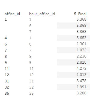
As you can see it is almost looking good but we need to remove those rows that are basically duplicates (rows two and three) or should not be on the view at all (row 4).

So, one little last thing to be done: creating a filter. Since a dimension filter will break everything we used above (since they calculate prior to table calcs, thereby effectively removing needed measure values and dimensionality) we have to turn the filter into a table calculation as well:

//Filter
lookup(min([office_id]),0) = lookup(min([hour_office_id]),0)

Put this in the filter shelf, set to true (compute table down) and you are done.

Summary

What is the thinking here?

First, we define via a ranking and a window_min of that ranking (calcs 1 and 2) on which rows we want to compute our calculations which is only the first row per (somewhat alike partitioning by row number in sql).

Then, we create the sum per hour_office_id (hour_office_id is our “window”, thus window_sum). Since calcs 1 and 2 are nested in 3, this is done only on the first row. This enables us to grab also values that are in other rows that do actually not belong to the office_id. We effectively create a sub-table that contains what we need and attribute that against the original table. This is where the actual thinking took place.

For calculation four we then need to go a long way to get things right but the essence is: define those values that we need to subtract, i.e. to remove from our value per office_id.

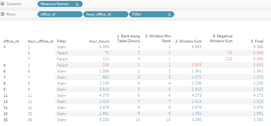
Calculation five is just bringing it all together and the filter is cosmetics. Below as a step by step result, highlighted in red those fields that the filter will hide.

Now this was a lot to take in and yes, there are alos other options, at least in this particular case like LODs (fellow Tableau user Kelsie Barnes answered with an LOD option) but I wanted to do it this way since the LODs are not necessarily any easier and the general technique can be applied to other requests as well as I will show in a follow up to this posting.

I hope you found this useful. and as always I appreciate your feedback.

Until next time

Steffen