How to do a count distinct over a rolling window

Recently a user on the forums asked how a distinct count over a rolling window could be done.

Easy, you might say at first. Just use countd() and all be good. And that is true – and it is not.

The problem we are facing here is that the usual countd() combined with say a quarterly time dimension will translate into (using bigQuery syntax)

SELECT
date_trunc([date field], QUARTER) as `date`,
count(distinct customer_name) as distinct_customers
FROM [your source]
group by 1

This will give us back the distinct count of customers within each quarter. But what if we want this info to be rolling three months?

I.e. in March we want the distinct count of customers from Jan to March and in April it would be Feb to April etc. What if we want this rolling window to also be dynamic?

The challenge

Your first guess might be to then simply do a countd() per month and then use a window_sum() function over that in which we specify the window.

i,e. something like this:

window_sum(countd([customer_name]), -[parameter or fixed value],0)

But the problem arises quickly.

Highlighted here is the result of such an approach when using three months rolling (including the current month). The sum of each month’s individual count distinct is 130.

But let us put this now to quarterly aggregation:

The actual distinct count of customers within these three months is only 123, not 130.

So what we need is a defined window onto which we then apply a count distinct.

Unfortunately, there is window_count() but no window_countD() in Tableau.

And count() will always be grouped by the granularity defined within our view, as laid out before.

How to overcome this problem?

Step 1 – a bit of data prepping

As usual, we will build on sample superstore. Our example will be limited to allowing a rolling window of max 12 months.

Connect to the data source, then drag the orders table onto your table canvas twice, such that you get a relationship.

Edit your relationship to be based on two conditions:

Notice that you can also do this using physical joins but be advised that your data source will blow up very (!) fast. The 10k rows of sample superstore become close to 23.5 million rows if you use the above on a join. Therefore, if you need to do a join it is highly recommended to first roll up your data to the date aggregation level you need.

In super store terms that would mean that we roll up from daily to monthly as the month is our intended level of granularity and then do the join.

In a nutshell: this is a prime example of where relationships truly shine.

With that prepared I created custom dates (right click your date field, select “custom date” –> month, keep at “date value” ticked) for both order date columns from table 1 and table 2. This is just easier than constantly using calculations.

Let us put these on the view and see where we stand:

Looking good.

Step 2 – just one filter needed

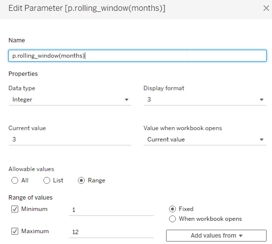
Before we do the calculations, go on and quickly create a parameter that will allow us to define the rolling window size (i.e. how many months back).

Next, we create one filter calculation and one further calculation. The second calculation is actually not needed and only serves on an intermediate testing phase. You can create it or leave it out from the get-go.

Create this filter:

//TF in rolling window
DATEADD('month',[p.rolling_window(months)]-1,[Order Date (Orders1) (Months)]) >= [Order Date (Months)]

Let’s put this on the view next to our two columns of order dates based on 3 months selected in the parameter

Result is what we hoped for.

Now, let us add the countd() of customers and besides that we will add this calculation:

//count distinct of customers in rolling window
{exclude [Order Date (Orders1) (Months)]: countd([Customer Name (Orders1)])}

Since – as per now – we still have two order dates in the view, we need to remove the granularity imposed by the second order date column. We do so using exclude.

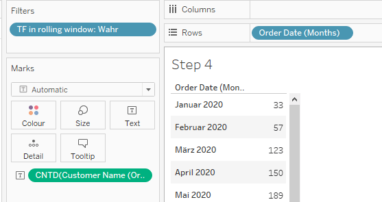
further, move the filter from the rows to the filter shelf and set to true.

Let us see what this gives us:

Isn’t this beautiful? In the first column we can see the distinct count of customers that are still grouped by the months as imposed by the view’s granularity. But the second column already shows what we want to see: 123 (see above when we discussed the problem).

For the last step, we can now even remove the [count distinct of customers in rolling window] calculation and also remove the [Order Date (Orders1) (Months)] from the rows.

The result will still be correct as the relationship is triggered by the filter. See March 2020 (sorry, I forgot to set my locale to English, but you will still get it I assume).

Let’s close out with some final Q&A. Here is the yearly distinct count of customers:

And here is what we get if we set our parameter to 12 and check on the December values for every year:

Simply beautiful, isn’t it?

And with that we are done.

I hope you found that useful and as always appreciate your feedback.

Until next time.

Steffen