Let’s build – fun with maps

In today’s episode of “Let’s build” we will create a dashboard (or: a sibling thereof) that I presented during our E&V Tableau Days 2023.

Given that during that session I only had 35 minutes to do the data source prep and explanations, the calculations (20+) and then the actual dashboarding, I was a bit under time pressure and here and there parts of the audience might have gone lost due to the speed I presented at.

So, let’s remedy this and build & explain everything from scratch.

Here is a glimpse at what we gonna build. Be advised that the gif depicts a more advanced version which is too much for a blog post.

We will be doing only the “first level”, i.e. map, bar chart, macro and micro zoom with headlines on top of them providing additional information. No diving into further details as is happening on the right (the bar chart will remain in full).

I have also prepared a “starter dash” that includes the data source and a calculated field with all the calcs in it so you can just drag and drop them. You can find it on my tableau public and use that as your starting point.

Part 1 – Building the data source

Our source consists of three parts:

1. An Excel table that contains all German cities including their identifier (LAU CODE), their region code (Schluessel, Key) with their latitude and longitude, enriched with some population data and also with the so called NUTS3 latitude and longitude – why the latter may be important we will see later on.
2. An excel list with shop locations – for this, I simply used file 1, added random numbers to all of them and selected the first top 300 to define which cities will be our “shop bearing cities”.
3. A spatial file for the area outlines of the map.

Parts 1 and 3 can all be found on the websites of the German Bureau of Statistics with some searching around and cleaning.

Part 2 is obviously just a subset of 1) and therefore you will automatically have it.

This is what our source will look like:

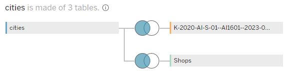
As you may figure, we are on the physical layer using classic joins, no relationships.

Why do we do that? Because for the shops with cities join, we will be using a spatial join which is not supported by relationships.

The join conditions are as follows:

For joining the K-2020… file which is our spatial file we can simply use a provided “Schluessel” (i.e. Key) column as its coming straight from the German Bureau of Statistics. Same for the cities, which have this information available.

For joining the shops with the cities, I opted for a spatial join. In order to be able to play around with the parameter, we need to join all shops with the cities.

Wait, all shops and all cities? That would be quite an overreach as there is no reason to join a city in the north of Germany with a fake super store shop in the south – no customer would travel 900km.

So, here is the join condition:

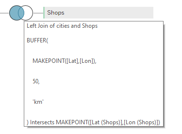
As you can see, we create a buffer around the cities, for which we calculate the individual geo-points based on the latitude and longitude, with a radius of 50km and check if the individual shops with their geolocation intersects this buffer.

The parameter we will use on our sheet is therefore also set to a maximum of 50kms as anything beyond that would return no additional rows from the data set.

Part 2 – The calculations

Shop and City calculations

We will now first create all the calculations we will be needing. It is gonna be quite a lot so bear with me.

Let’s start with

//shop_point
MAKEPOINT([shop_lat],[shop_lon])

followed by

//city_point
MAKEPOINT([Lat],[Lon])

With these, we have turned the lat and lon fields from our data sources into geo points that tableau can plot on a map. So far, so good.

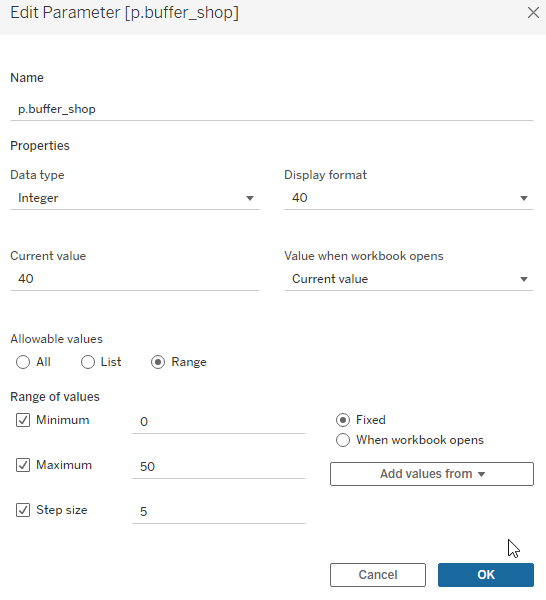
Next on the menu is to create a parameter named p.buffer_shop, set as integer allowing a range of 5-50 as we will need it in the following calculations. This parameter is the one that allows us to play around with how far our customers must travel to find the next shop.

Now that we have this set up, on to the next calculation:

//buffer around shops
BUFFER([shop_point],[p.buffer_shop],'km')

Here, we create a radius around our shops. Based on the afore create shop_point, we can now use the parameter to define the radius that Tableau will draw around them.

And this allows us to create the next step:

//intersect shop/city
IF INTERSECTS([city_point],[buffer around shops]) then 1 else 0 end

Here, we test if our cities intersect with the just created buffer around our radius. If so, we return 1 and if not, 0.

For our tooltip, we also want to know the distance to the (nearest) shop:

//Distance shop from city
DISTANCE([city_point],[shop_point],'km')

This simply returns for every shop and city the distance between them, limited of course to those pairs that made it through our initial join in the data source (so: 50km is the maximum distance we will ever find, anything beyond that is null).

The next calculation will need some explanation. The [Area id] is the key for each of the 400 German areas, it’s unique identifier. The [LAU CODE] field is the same just for cities / communities in Germany.

//number of cities in range per area
{fixed [Area Id]: COUNTD( if [intersect shop/city] = 1 then [Lau Code] end)}

What this calculation does is to return to us the distinct count of [Lau codes] (aka Cities) that have an intersection with at least one shop. We are using distinct count here because one city might intersect with more than one shop and we do not want to double count those. In effect, we now know how many cities within each area are having a “touching point” with at least one shop.

Next, we also need to know the number of cities within each area in general. The calculation is the same as before, just leaving out the if condition.

//number of cities per area
{fixed [Area Id]: COUNTD([Lau Code])}

And with these two established, we also have at hand the number of cities we are missing.

//number of cities missed
[number of cities per area] - [number of cities in range per area]

We close out this section of the calculations with calculating the population per city.

//Population per City | FIXED
{fixed [Lau Code]: avg([Population])}

Here, we essentially remove the duplication effect that stems from our spatial join. Why is that? Well, if a city has touchpoints with more than one shop, this will create one row per combination in the data source like

city –> shop a

city –> shop b

And since city has the population information attached, we need to average it for every lau code (aka city) . If our city has 200k inhabitants and two shops are within 50kms, summing the population would give us 400k which is false. Averaging it gives us the 200k we expect since average of 2x200k is 200k.

Area calculations

Continuing now with the area related calculations we kick it off with creating three calcs that we need to create our macro zoom (the zoom on the upper left which zooms in but leaves room to show a bit of the area’s surroundings).

Start by again creating a parameter:

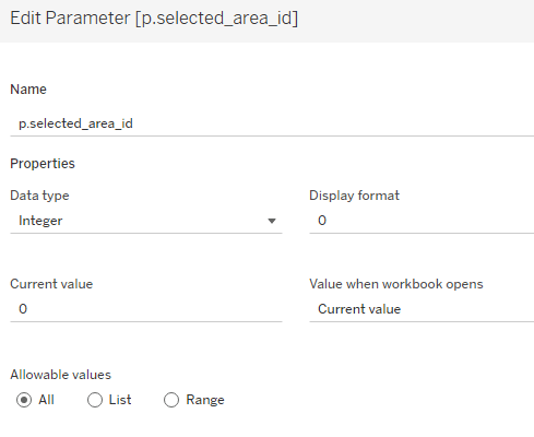
then, on to the calculations:

//Selected area lat
if [p.selected_area_id] = [Area Id] then [NUTS Lat] END

and

//Selected area lon
if [p.selected_area_id] = [Area Id] then [NUTS Lon] END

These two return to us the latitude and longitude of the areas (their center points), not the shapes. The shapes come from our joined shape file and do not require any further calculations.

With the two afore calcs we can now create the buffer calculations around our areas. If nothing is selected in our parameter that is going to hold the area_id depending on what the user clicks, then we will create super tiny buffers around every area. This is needed because if we do not do that, Tableau will do some crazy zooming out if nothing is selected. There is another option we can use but for now, let’s stick with this one.

If something is selected, we will go for a 50km zoom around the central point of our selected area

//Buffer around selected area
IF [p.selected_area_id] = 0
THEN
BUFFER(MAKEPOINT([NUTS Lat],[NUTS Lon]),0.005, 'km')
ELSE
BUFFER(MAKEPOINT([Selected area lat],[Selected area lon]),50, 'km')
END

Further, we need to know if an area is the one that was selected:

//TF is selected area
[p.selected_area_id] = [Area Id]

And if it is, we want to label it

//Label selected area
IF [TF is selected area] THEN [Area Name] END

One more calculation and we are done with our area related calculations:

//coloring area
IF [number of cities in range per area] = 0 THEN 'uncovered'
ELSEIF [number of cities per area] > [number of cities in range per area] then 'partially covered'
else 'fully covered'
END

Here, we create a dimension with three members to be able to easily select three colors for those areas that are fully covered (every city in the area has at least one shop in range), partially (only some cities have touchpoints) or uncovered (no city has a shop in range)

Calculations for our headlines

First, we need to population of Germany to be able to later on calculate the percentage we are missing

//Population Germany
{sum([Population per City | FIXED])}

Why can I now use sum in this table-scoped fixed LOD? Because we have taken care of deduplicating the measure results earlier on in our population per city calculation. So, now we can simply sum up all the (deduped) populations and will have the German population.

The next one may need some additional explanation

//missed population per city considering intersect | include
{include [Lau Code]: avg([Population])*  (1-max([intersect shop/city]) ) }

The reason to include the LAU Code field (i.e. the city identifier) is that we use this calculation on our bar chart where we will not have the LAU Code present. But we need it in order to evaluate city by city of the city is touched or not. If it is, the last part of the calc will be 1 – 1 (remember? we had the result of our intersect check calculation to be 1 and 0 instead of true/false. This is why. So, 1-1 = 0 multiplied by the population will give 0 again which means for this city we will not sum the population as missed (which is correct, because the city is in range).

For all other cities, the calculation will for example give

“For LAU CODE 01305800: 200,000 (avg pop) * (1- max of (0,0,0,0 = 0) –> 200,000 * 1 = 200,000 = missed population for this city.

For the headline, we need to turn this also into a window calculation to basically eliminate the LAU Code effect (otherwise, in the header our calculation would show 10,000 to 900,00 or something like that. So, the min and max ends of the range.

//missed population per city considering intersect | TC WinSum 
window_sum(SUM([missed population per city considering intersect | include]))

Next, we need to know the population per area:

//Population per Area | FIXED
{FIXED [Area Id]: sum([Population per City | FIXED])}

Here we say: for every area id, give me back the sum of the population per city.

Finally, since our info of what percentage we are missing is put on top of the bar chart

//Population PCT missed total (bar chart) | TC 
[missed population per city considering intersect | TC WinSum] / sum([Population Germany])

Here, we divide the sum of the missed population by the sum of the german population.

Final calculations

To close out this section, we need two more calculations as we want to dynamically show and hide parts:

//dynviz show detail
[p.selected_area_id] != 0

If the parameter is not equal to zero, then it means something has been clicked and we want to show the details. (The calculation is true)

On the opposite end, we want to hide parts when we are showing details:

//dynviz no detail
NOT [dynviz show detail]

So, now let’s get into the actual dashboarding

Creating the sheets and dashboard

Map (incl Macro zoom)

Start of by creating the map. Drag the geometry field onto the canvas. Then, drag [Area Id] onto details to split the individual German areas.

Put [coloring area] on the colors, assign green to fully covered, grey to partially covered and red to uncovered.

Put [Label selected area] on the labels mark

Next, drag [buffer around selected area] onto the viz as new map layer:

Now, we want to also show the shops, so take [shop_point], drag it again as a new layer onto the map. Split it by putting [shop_name] onto the details. Change the mark type to “shape” and select whatever you like. For coloring, this is up to you. I suggest taking something light.

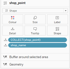
To finalise, click on the small downward triangle next to the layer names

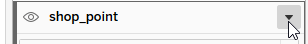
For shop point and geometry layer, untick “add to zoom extent”. For the buffer, tick “hide” as we only want to use it but not see any buffer. Keep “add to zoom extent” ticked for the buffer layer.

Zoomed map (micro view)

Go to a new sheet, add [TF is selected area] on the filter shelf but do not set to true yet.

Create geometry layer as before, geometry on viz canvas, area id on details.

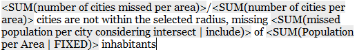
Add [number of cities missed], [number of cities per area], [missed population per city considering intersect | include] and [population per area | fixed] onto the details as we will need these in our header

double click the title and adjust like this:

Add now our [city_point] just as we did for the shops before as a new layer, split it by using [LAU Code] on the details

Add our [intersect shop city] onto the colors, change from sum to max and make it discrete.

You may wonder why we need to turn it into max. See here

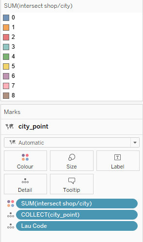
As several cities have more than one shop, sum would give us a range. But we are only interested if at least one shop is in range, so we go for the max of the intersect and since intersect is either 0 or 1, the max will be one. And we get a nice split that we can use for is in range (Green, 1) or not in range (0, red).

also feel free to add the [lau name national] field onto the tooltip.

Change the mark type to circle and drag the[ population per city] field on the size

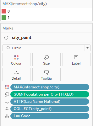
Finally, set the filter on the filter shelf to true.

Last Chart – Bar chart

For our last chart, put [area id] and [area name] on the rows.

Add sum([missed population per city considering intersect | include]) on the columns.

This chart is why we need the include function in our field since – as you will notice – nowhere else on this chart are we referencing the cities (or their lau codes)

Add our [coloring area] field onto the filter and remove “fully covered”. Add it also onto the colors. Sort the bars.

Double click on the marks area to open an ad-hoc calculation field. Put size() in it.

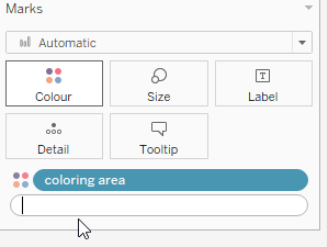
Add [Population PCT missed total (bar chart) | TC] and [missed population per city considering intersect | TC WinSum] on the details as well.

All of these three are window or table calculations. Click them, go to edit table calculation. Select “specific dimensions” and make sure all three are ticked.

Edit the sheets title to this:

Remove show header from the area id and the axis.

And with that, we have all our three sheets done.

Dashboarding & Actions

Go to your dashboard and add the sheets in a fashion you like.

I’d suggest to split your layout into left and right and on the left, use a vertical container that splits your map and your micro level map

Select the zoomed map, click layout and “control visibility using”. Select [dyn viz show detail]

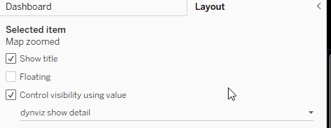
Show the radius selector parameter and then use the other dynviz field to hide it when we are showing details

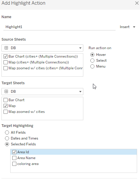
Now, go to Dashboard –>Actions and add a highlight action. Use the bar chart as the source, the map as the target and area id as the field

Add our second action, the area selection action:

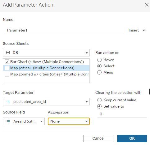
Make sure to select “set value to” –> 0 as otherwise our calcs will break at some points.

And that’s it for today.

I hope you found that useful and as always, appreciate your feedback.

Until next time.

Steffen