LODs, Row Level Permissions, Cross joins and potentially a whole lot of costs

Today I have something that is related to optimizing your dashboards and/or data source row level permission for cost savings and to raise awareness of something that maybe you are not really aware.

We will be looking into the effects of using (table scoped) LODs in combination with row level permission filtering at the source.

At the source here means that your row level permission determinator is included already directly into your data table.

In this testing case, the RLP column consisted of all user right strings concatenated like so:

RLP	Dimension member	Measure value
UserA | UserB | UserC	A	56
UserA | UserC	B	12
UserA | UserB | UserD	C	34

Let’s see what Tableau makes of this and how this significantly increases query complexity and your costs.

Obviously, we will also see if there are ways to mitigate this.

The test environment

• google bigQuery connector, not the 2023.1 JDBC but original
• live connection
• Source: 36m rows of daily data
• Target: a simple table
• Source filtering includes RLP where the RLP is based on a concatenated string that is queried using contains( [username], USERNAME() )
• Two LODs as part of two other calculations,both being { max([Date]) } –> table scoped LOD

1. BASE LINE case

In order to set our comparison base line, my first try was using a file that included the two table scoped LODs but did not apply inbound rlp.

This is the table we are looking at (sorry I have to obfuscate quite a bit but that does not really matter)

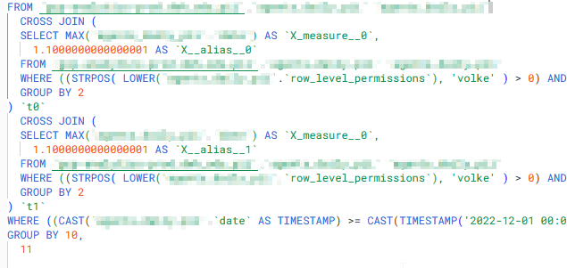
Here is an extract of the resulting query

Notice the two cross joins at the end?

These are the two table scoped LODs { max([Date]) } within my two calculations. Also notice how the resulting max date is not only cross joined (which makes sense because an LOD basically provides this invisible extra column) .

2 Adding RLP

Now, if we add our RLP directly in the data source, using the existing username column we get almost the same query but within the two LOD related cross joins, we see the querying of also the row level permissions.

Visualised we see this:

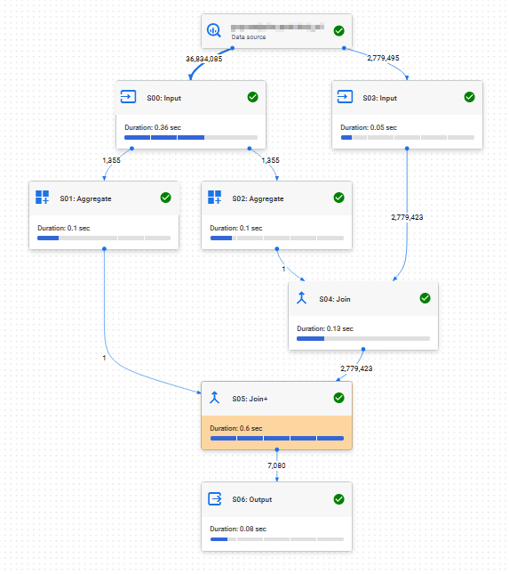
Right hand part is the “actual” query whereas on the left, quering the 36m rows are the LODs. The results running the query directly in google cloud console where these:

Version	Queries	Processed	Elapsed time	Slot time consumed
Base LOD, no RLP	1	563mb	1 sec	102 secs
LODs, inbound RLP	1	23,45 GB	1 sec	105 secs

Removing one of the LODs does reduce the cross joins, but that is about it. No change to processed GB (which is expected).

3 REPLACING LODs WITH TODAY()

Next, I tried replacing my LOD with a simple today() formula instead. Obviously, this may not be for every case but still I wanted to check on it.

We kept the RLP filtering as it was (contains… username..)

Let’s add this to our results table

Version	Queries	Processed	Elapsed time	Slot time consumed
Base LOD, no RLP	1	563mb	1 sec	102 secs
LODs, inbound RLP	1	23,45 GB	1 sec	105 secs
Today, inbound RLP	1	1,51 GB	1 sec	29 secs

So, what we notice is that w/o our LODs and thus the multiple runs of RLP checking we process significantly less data.

4 CHANGING RLP TO RELATIONSHIP

Now, for the next try we change our RLP. Instead of using the inbound RLP column with “contains(…)” function, we put another data source to our main data source and relate them.

The newly related RLP data source differs in such a way that it has one (1) row per user and allowed id. I.e. a 1:1 ratio meaning a user with access to 100 ids will have 100 rows in the RLP source.

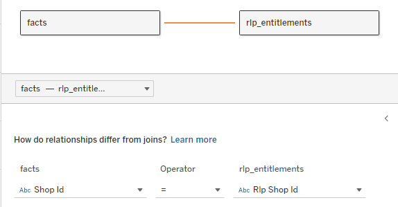
The RLP filter is now changed to

 [RLP Username] = username()

The result is two queries which is to be expected and we can see the inner join that results from the relationships:

Results are documented here (considering both created queries):

Version	Queries	Processed	Elapsed time	Slot time consumed
Base LOD, no RLP	1	563mb	1 sec	102 secs
LODs, inbound RLP	1	23,45 GB	1 sec	105 secs
Today, inbound RLP	1	1,51 GB	1 sec	29 secs
LODs, relationship RLP	2	3,43 GB	2 sec	260 secs

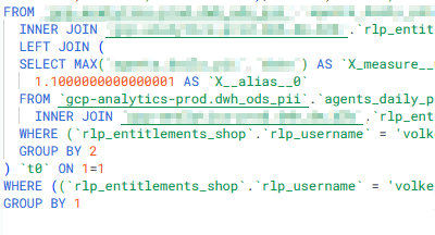
5 Physical join

For this test I went to thy physical layer and created a classic inner join of the data source, then applying the same RLP logic of

[RLP username] = username()

Adding test results:

Version	Queries	Processed	Elapsed time	Slot time consumed
Base LOD, no RLP	1	563mb	1 sec	102 secs
LODs, inbound RLP	1	23,45 GB	1 sec	105 secs
Today, inbound RLP	1	1,51 GB	1 sec	29 secs
LODs, relationship RLP	2	3,43 GB	2 sec	260 secs
LODs, physical join RLP	1	1,85GB	1 sec	102 secs

6 Physical join with today

Sticking with the physical join but swapping my LODs for a simple today() has a significant effect

Version	Queries	Processed	Elapsed time	Slot time consumed
Base LOD, no RLP	1	563mb	1 sec	102 secs
LODs, inbound RLP	1	23,45 GB	1 sec	105 secs
Today, inbound RLP	1	1,51 GB	1 sec	29 secs
LODs, relationship RLP	2	3,43 GB	2 sec	260 secs
LODs, physical join RLP	1	1,85GB	1 sec	102 secs
Today, physical join RLP	1	132 MB	0,5 sec	33 secs

7 Relationship RLP and today()

For the final exercise, let’s also check on combining relationship-based RLP using today() instead of our LODs.

Version	Queries	Processed	Elapsed time	Slot time consumed
Base LOD, no RLP	1	563mb	1 sec	102 secs
LODs, with RLP	1	23,45 GB	1 sec	105 secs
Today, with RLP	1	1,51 GB	1 sec	29 secs
LODs, relationship RLP	2	3,43 GB	2 sec	260 secs
LODs, physical join RLP	1	1,85GB	1 sec	102 secs
Today, physical join RLP	1	132 MB	0,5 sec	33 secs
Today, relationship RLP	2	1,96 GB	1.6 sec	111 secs

And this concludes our little trip into LODs, Row Level Permissions and potentially associated costs.

Summary

Based on what we tried, the key take-away are:

1. Make sure to not use any table scoped LODs that you do not really need if RLP is in place.
2. If you need (for user experience) to calculate the max date as a starting point for a parameter, consider moving that calculation directly into your data source
3. If you are creating something that will have a foreseeable high load, try out different versions of it if you can. The results can be significantly different, as you can see above.

More things to be checked

1. I could not find if Tableau caching would maybe speed up / remove querying needs for any further usage of the max(date) LOD
2. Could ordering the base table do any good?
3. Clustering, indexing of the base table, what are the effects?

These unfortunately are things that are a bit beyond me (I am a finance guy, after all) but I will try to generate some more insights and in case I manage will be adding the findings.

That’s it for today, I hope you found that useful.

As always, appreciate your feedback.

Until next time.

Steffen